The March 29, 2006 Total Solar Eclipse

On Wednesday, March 29, 2006, a solar eclipse was visible in the northern hemisphere. A total eclipse occurred within a narrow corridor starting near the equator in the Atlantic Ocean, crossed central and northern Africa, went across the Mediterranean Sea to Turkey, and terminated at sunset in central Asia. Maximum eclipse occurred in the southern desert of Libya, lasting 4 minutes and 7 seconds. The eclipse was visible in Egypt near the Libyan border at 10:40 UT (12:40 local time) with a duration of 3 min 58 sec, and near Antalya in Turkey at 10:57 UT (13:57 local time) with a duration of 3 min 45 sec. For a detailed description of the eclipse path, see NASA’s Eclipse page. For useful information about eclipse photography, see Fred Espenak’s Eclipse web site.
On March 12, 2006, we initiated an MHD computation of the solar corona, in preparation for our prediction of what the solar corona would look like during this eclipse. We used photospheric magnetic field data measured up to March 10, 2006, by the MDI magnetograph aboard the SOHO spacecraft. We typically also use magnetic field measurements from the Wilcox Solar Observatory at Stanford and the National Solar Observatory SOLIS vector magnetograph at Kitt Peak.
A preliminary prediction of the state of the solar corona during the eclipse based on this data was published on this web site. This preliminary prediction can be found here. On March 18, 2006 we started a new calculation with updated magnetic field data that was measured with MDI up to March 17, 2006. This page has the updated (and final) prediction, which was posted on March 24, 2006.
This year we significantly improved our coronal modeling capability. In the past we used the “polytropic” model to describe the flow of energy in the corona. This is a crude model of the corona that greatly simplifies the calculations. In recent years we improved the energy equation in our model to include the effects of coronal heating, the conduction of heat parallel to the magnetic field lines, radiative losses, and the effect of Alfvén waves. This produces a significantly better estimate of the plasma temperature and density in the corona. For technical details about our improved model, please see the publications below. The prediction shown here uses our new model, and allows us to predict emission in extreme ultraviolet (EUV) wavelengths and X-rays, which can be compared with solar observations from the EIT imager on SOHO and the X-ray instrument on Yohkoh (no longer operational), in addition to emission in polarized white light (polarization brightness, pB) that is typically measured during an eclipse.
A comparison between our prediction and several eclipse observations is on the original comparison page.
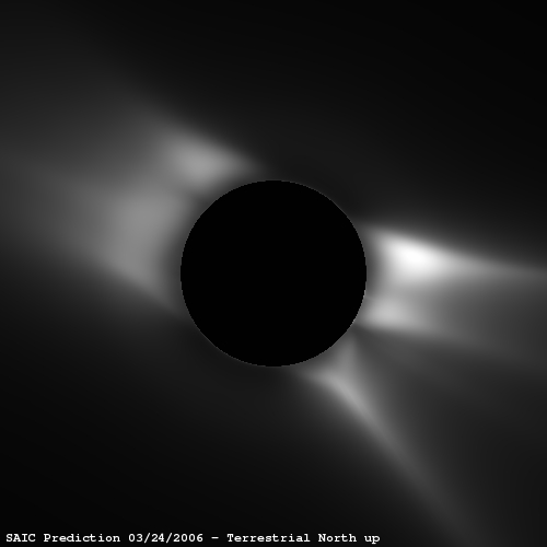
Predicted polarization brightness (pB) in the solar corona for the eclipse expected on March 29, 2006 at 10:57 UT (corresponding to totality near Antalya, Turkey). The state of the solar corona was computed using a 3D magnetohydrodynamic (MHD) simulation. The pB signal is produced by white light scattered off electrons in the coronal plasma. The image has been radially detrended using the Newkirk vignetting function to account for the fall-off of coronal brightness with distance from the Sun. Vertical (top) is terrestrial (geocentric) north. This is the view of the Sun that would be seen by an observer on Earth with a camera aligned so that vertical is toward the Earth’s north pole. Views aligned with solar north are on the original solar-north page.
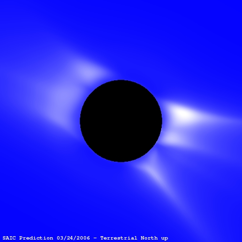
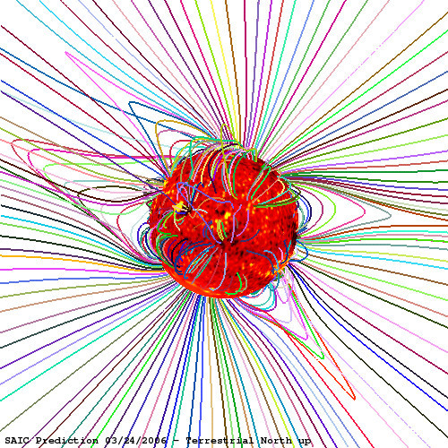
Predicted polarization brightness (left) together with traces of the magnetic field lines in the solar corona (right) for the eclipse expected on March 29, 2006 at 10:57 UT (with terrestrial north up). The Sun’s surface shows color contours of the radial component of the measured photospheric magnetic field from the MDI magnetograph, showing the location of active regions (strong magnetic fields).
Evolution of the Photospheric Magnetic Field
The photospheric magnetic field maps we use for our calculations are built up from daily observations of the Sun during a solar rotation. These maps give a good approximation of the Sun’s magnetic flux if the large-scale flux is not changing much throughout a rotation. Previously, we have computed coronal models for an eclipse during the declining phase of the last solar cycle (November 3, 1994), for two eclipses during solar minimum (October 24, 1995 and March 9, 1997), one eclipse during the early rising phase of solar cycle 23 (February 26, 1998), one eclipse approaching solar maximum (August 11, 1999), and two eclipses near solar maximum (June 21, 2001 and December 4, 2002).
The March 29, 2006 eclipse occurred near solar minimum, so the solar corona ought to (and does) have a simpler structure than at solar maximum. It can be seen that the solar corona is most similar to that seen in the eclipses near solar minimum on November 3, 1994, October 24, 1995, and March 9, 1997.
CR2037 (Nov 25 – Dec 22, 2005)
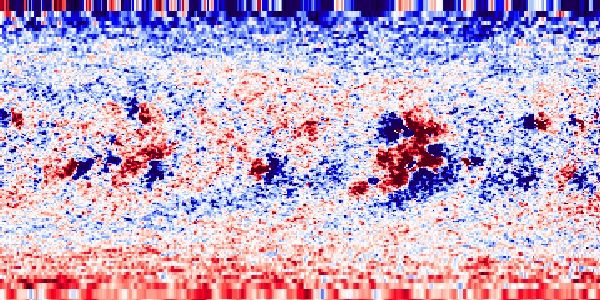
CR2038 (Dec 22, 2005 – Jan 18, 2006)
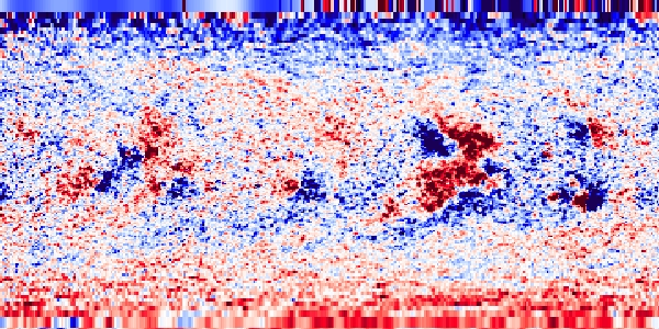
CR2039 (Jan 18 – Feb 15, 2006)
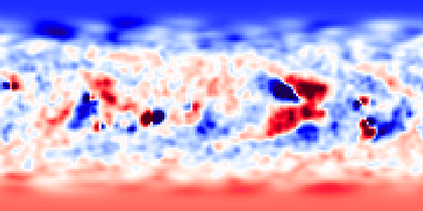
CR2040+CR2041 (Feb 18 – Mar 17, 2006)
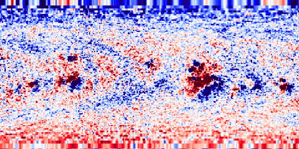
These figures show the evolution of the solar photospheric magnetic field for three Carrington rotations preceding the eclipse, as measured by the SOLIS vector magnetograph at the National Solar Observatory at Kitt Peak, and one rotation from the MDI magnetograph aboard the SOHO spacecraft. This last rotation, which contains data measured from February 18 through March 17, 2006, and includes parts of Carrington rotations 2040 and 2041, was the data used in our calculation for the updated eclipse prediction; this calculation was started on March 18. The maps show the measured photospheric magnetic field as a function of latitude (vertical axis) and Carrington longitude (horizontal axis). Red shows outward directed magnetic flux, and blue shows inward directed flux.
Coronal Emission
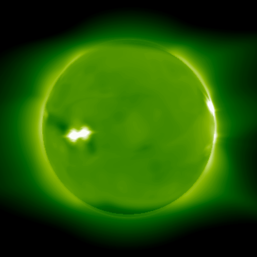
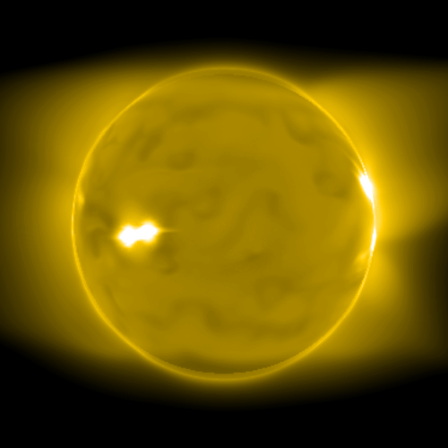
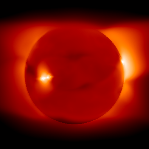
We compute emission of radiation from the corona by integrating the emission kernels for extreme ultraviolet (EUV) and X-ray radiation along a chosen line of sight. This integration requires knowledge of the plasma density and temperature in the corona, which we predict using our model. The images below show the predicted coronal emission at the time of the eclipse.
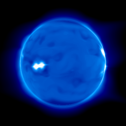
EUV 171 Å Emission
EUV 195 Å Emission
EUV 284 Å Emission
X-Ray Emission (Al/Mg Filter)
Predicted coronal emission at the time of the eclipse in three EUV wavelengths and in soft X-rays.
The corresponding emission movies, which illustrate how the emission changes as the Sun rotates:
EUV 171 Å Emission
EUV 195 Å Emission
EUV 284 Å Emission
X-Ray Emission (Al/Mg Filter)
Movies of Polarization Brightness
We have made movies of the polarization brightness (pB) from our MHD simulation. This illustrates visually how the solar corona changes as a result of solar rotation. The left movie shows pB with an image of the radial magnetic field on the Sun’s surface; the right movie shows pB with a black disk occulting the Sun.
Polarization Brightness(with surface magnetic field)
Polarization Brightness(with occulting disk)
Publications
For technical details about our model, please see the publications:
- Z. Mikić, J. A. Linker, D. D. Schnack, R. Lionello, and A. Tarditi, “Magnetohydrodynamic Modeling of the Global Solar Corona,” Physics of Plasmas, 6, 2217 (1999).
- Z. Mikić, J. A. Linker, P. Riley, and R. Lionello, “Predicting the Structure of the Solar Corona During the 11 August 1999 Total Solar Eclipse,” in The Last Total Solar Eclipse of the Millennium (W. Livingston and A. Ozguc, eds.), ASP Conference Series, Vol. 205, p. 162 (2000). Download PDF
- Z. Mikić, J. A. Linker, R. Lionello, P. Riley, and V. Titov, “Predicting the Structure of the Solar Corona for the Total Solar Eclipse of March 29, 2006,” in Solar and Stellar Physics Through Eclipses (O. Demircan, S. O. Selam, and B. Albayrak, eds.), ASP Conference Series, Vol. 370, p. 299 (2007). Access Article
Acknowledgements
Our work is supported by NASA’s Sun-Earth Connection Theory Program (SECTP), Supporting Research & Technology (SR&T) Program, and Living With a Star (LWS) Program, and by the Center for Integrated Space Weather Modeling (an NSF Science & Technology Center). We thank the staff at the San Diego Supercomputer Center (SDSC) for providing us dedicated time on the DataStar supercomputer for timely completion of our calculations. We also thank NASA’s Advanced Supercomputing Division (NAS) for an allocation on the Columbia supercomputer, on which many of our runs have been performed. We thank Yang Liu and Todd Hoeksema of Stanford University for providing us with timely access to the MDI magnetograph data and for sharing their latest calibrated data with us.
Archived prediction, converted from the original 2006 page. Movies originally offered as GIF/QuickTime downloads are embedded above.